15 Traffic Flow Forecasting
15.1 Spatio-Temporal Graph Convolutional Networks (STGCN)
These notes refer to the conference publication B. Yu (2018) code implementation is provided at github.com
15.1.1 Graph Convolutions
Similar to ASTGCN presented in Section 15.2, STGCN utilizes graph convolutions and temporal convolutions in order to compute spatial correlations in the graph data representations.
The graph convolution operator, “*_{\mathcal{g}}” is used for identifying the spatial correlations in the data:
\Theta *_{g} x = \Theta(L)x = \Theta(U \Delta U^{T})x = U\Theta(\Delta)U^{T}x
Again, the graph Fourier basis U \in \mathbb{R}^{n\times n} is used in order to transform the computation space of the convolution to the spectral space. This Fourier basis is the matrix of eigenvectors of the normalized graph Laplacian L. See this lecture on the normalized Laplacian matrix for more information …
L = I_{n} - D^{-\frac{1}{2}}WD^{-\frac{1}{2}}
15.1.1.1 The Normalized Laplacian
Important Definitions:
- multiset: a generalization of the concept of a set. Unlike a set which allows for only one instance of each of its elements, a multiset may contain multiple instances of the same element. The number of times a given element appears in the multiset is known as its multiplicity. As with normal sets, the order of elements is not relevant.
- cardinality: the sum of multiplicities for all elements (number of items)
Spectral Graph Theory
- What are the relationships between the structure of a given graph and the eigenvalues of a matrix associated with the graph?
- Ajacency matrix: indicates which vertices are adjacent. Eigenvalues can count closed walks, so can count edges and test bipartite-ness
- Laplacian L=D-A: positive semi-definite. Eigenvalues can count edges and number of components
- Signless Laplacian Q = D + A: unsigned incidence matrix, positive semi-definite. Eigenvalues can count edges and number of bipartite components
- Normalized Laplacian \mathcal{L} = D^{-1/2}(D-A)D^{-1/2}: normalizes the Laplacian matrix, and is tied to the probability transition matrix
- eigenvalues \in [0,2]
- multiplicity of 0 is number of components
- multiplicity of 2 is number of bipartite components
- tests for bipartite-ness
- cannot always detect number of edges
Normalizing matrices is useful.
15.1.2 Network Architecture
Components:
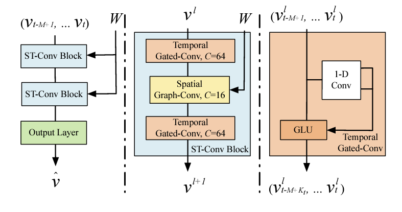
- two spatio-temporal convolutional blocks (ST-Conv Blocks) and FC output layer \rightarrow \hat{V}
- residual connections and bottlenecks are applied within each block
- ST-Conv Blocks contain
- one spatial graph convolution layer (in the middle)
- two temporal gated convolution layers
Graph CNNs for Extracting Spatial Features
Because the kernel computation \Theta in the graph convolution can be expensive due to O(n^{2}) multiplications with grpah Fourier basis, approximation strategies are utilized:
- Chebyshev polynomial approximation
- 1st-order approximation
15.1.3 Graph Convolution Approximations
Chebyshev Polynomials Approximation
- chebyshev polynomials are used in order to reduce the numebr of parameters required by the kernel \Theta.
- Chebyshev polynomials usually approximate kernels as truncated expansion of order K-1 \Theta(\Delta) = \sum_{k=0}^{K-1}\theta_{k}T_{k}(\tilde{\Delta})
- \tilde{\Delta} = 2\Delta/\lambda_{max} - I_{n}
- \lambda_{max} is the greatest eigenvalue of the Laplacian matrix
- Mathematical formulation for the graph convolution: \Theta *_{g} x \sim \sum_{k=0}^{K-1}\theta_{k}T_{k}(\tilde{L})x
- T_{k}(\tilde{L}) \in \mathbb{R}^{n \times n} - k\text{th} order Chebyshev polynomial, evaluated at the scaled laplacian, \tilde{L}
First Order Chebyshev Approximations
- first order approximation is used
- allows for a deeper architecture to be used
- not restricted to a specific parameterization by the polynomials
- scaling / normalization in Neural Networks ensure \lambda_{max} \sim 2
- assumptions simplify the graph convolution operation: \Theta *_{g}x \sim \theta_{0}x - \theta_{1}(D^{-1/2}WD^{-1/2})x
- \theta_{0} and \theta_{1} - shared parameters of the kernel
- W and D are also renormalized
- What does the D matrix indicate?
15.1.4 Gated CNNs - temporal feature extraction
- prior art uses RNNs (RNN-based models)
- RNNs have several critical limitations:
- time-consuming iterations
- slow response to dynamic changes
- complext gate mechanisms
- convolutional structures employed in entirety on time axis to capture temporal behaviors of traffic flows
- convolutions are faster for training
- allows for forming hierarchical representations
- each node of the graph, g, temporal convolutions explore K_{t} neighbors without padding
- reduces length of sequences by K_{t} - 1 each time
- I don’t have any idea what this means though …
- inputs to temporal convolutions - length- m sequences with C_{i} channels, Y \in \mathbb{R}^{m \times C_{i}}
- reduces length of sequences by K_{t} - 1 each time
- Definition of gated temporal convolution: \Gamma *_{\tau} Y = P \odot \sigma(Q) \in
\mathbb{R}^{M - K_{t} + 1} \times C_{0}
- is generalizable to the 3D convolution
15.1.5 Spatio-Temporal Convolutional Block
- (spatial) graph convolutions are combined with gated (temporal) convolutions
- temporal -> spatial -> temporal
- residual connections applied for improved training / avoid overfitting
- layer normalization used to prevent overfitting too
- General expression: v^{l+1} = \Gamma^{l}_{1} *_{\tau} \text{ReLU}(\Theta^{l}
*_{g}(\Gamma_{0}^{l} *_{\tau} v^{l}))
- \Gamma_{0}^{l} - upper temporal kernel in block l
- \Gamma_{1}^{l} - lower temporal kernel in block l
- \Theta^{l} - spectral kernel of graph convolution
- full structure:
- 2 ST-Conv Blocks
- 1 Temporal Convolution
- Fully connected layer to outputs
15.1.6 Prediction Task
- goal - predict speeds of cars for each of n nodes
- loss - L2 loss function
15.1.7 Experimental Evaluation / Study
Datasets
datasets contain key info of traffic observations / geographic information with corresponding timestamps
- BJER4 - Beijing Municipal Trafic Commission
- PeMSD7 - California Department of Transportation
Data Cleaning
- linear interpolation used for imputation
- data inputs normalized (z-score method)
Data Formatting
- separate methods are utilized in order to convert traffic data into the proper format for graph network analysis.
15.1.8 Topic Study Shortlist
- gated sequential convolutions
- what does it mean for these convs. to be gated? [DONE]
- what are chebyshev polynomials and how are they used to approximate convolutions?
- what are first-order approximations of the graph laplacian (see page 3 of STGCN paper) - kipf and welling 2016
- what does it mean for graph convolutions to be stacked vertically as opposed to being computed horizontally like traditional convolution operations
- what are gated linear units? (GLU) for non-linearity
- waht is linear interpolation imputation?
actually, understanding the theory behind these mechanisms is not especially relevant for my work. I simply need to know what the approximation is that they used for their computations. i.e. - we need to know the results, not how they were obtained.
15.1.9 What are Gated Convolutions?
Notes based on article from serp.ai
- Gated Convolutions - specific type of convolution that include a gating mechanism
- a sigmoid activation function determines which part of the input should be passed to the output and which parts should be “gated” or suppressed
Process
- input is convolved with a filter (like a regular convolution)
- before the result is generated, the input (after convolving) is passed through the gating mechanism
- sigmoid activation determines the part of the input are passed to the output, and which are suppressed (hence gated)
- use zero-padding - ensure output only depends on past inputs and doesn’t depend upon future inputs.
- this strategy might imporove interpretability - it may be easier to understand why certain predictions are made based on the results of the gating mechanism
- no activation is further applied after the gating mechanism has run
Gated Convolutions in STGCN
- Gated convolutions used in the Temporal Convolution Layer
- when the activation function (gating mechanism) is the “GLU”, the following formula is used: $$(x_{p} + x_{in}) (x_{q})
15.1.10 Approximated Convolutions (Chebyshev Polynomial Approximations)
Notes based on the youtube video Convolutions and Polynomial Approximation by kieransquared
- Approximations - finding a sequence of polynomials, P_{1}, P_{2}, P_{3} such that P_{n} converges to f
- An introduction to spectral graph theory
- spectral graph theory is based on the idea that specific properties of a given graph can be extracted from the eigenvalues, or approximate eigenvalues of a given adjacency or laplacian matrix representation of a graph.
15.1.11 What is linear interpolation?
- imputation method which assumes a linear relationship between missing and non-missing values.
- Assume you have three points, A, B, and X with features a and b (all have the same features). for A and B, the value of a and b are known, but for X, only the value of a is known. in this case, the missing value is calculated as the line between A and B, say f(x), such that f(x) = \frac{A_{b} - B_{b}}{A_{a} - B_{a}}x + c and c is some constant (intercept or bias). Then, X_{b} is approximated by f(X_{a}) \sim X_{b}
- Alternatively, some more specific linear interpolation polynomial can be specified.
15.2 Attention Based Spatial-Temporal Graph Convolutional Networks for Traffic Flow Forecasting
In this paper, S. Guo (2019) proposed a method for traffic flow prediction which utilized an attention based spatial-temporal graph convolutional network. They aimed to model several time-dependencies: (1) recent, (2) daily-periodic, and (3) weekly-periodic dependencies. The attention mechanism captures spatial-temporal patterns in the traffic data and the spatial-temporal convolution is used to capture spatial patterns while standard convolutions describe temporal features.
15.2.1 Core Contributions of ASTGCN
Difficulties of the traffic forecasting problem
- it is difficult to handle unstable and nonlinear data
- prediction performance of models require extensive feature engineering
- domain expertise is necessary
- cnn - spatial feature extraction from grid-based data, gcn - describe spatial correlation of grid based data
- fails to simultaneously model spatial temporal features and dynamic correlations of traffic data
- The convolution component of the network is meant to capture the neighborhood feature context surrounding each node - in a spatial temporal model, this means that a three dimensional kernel is required to account for the time dimension
- the spatial-temporal influence of different edges / connections between nodes varies across different time points.
Addressing these issues:
- develop a spatial-temporal attention mechanism
- learns dynamic spatial-temporal correlations of traffic data
- temporal attention is applied to capture dynamic temporal correlations for different times
- the attention mechanism learns the
- Design of spatial-temporal convolution module
- has graph convolution for modeling graph structure
- has convolution in temporal dimension (kind of like 3-d convolution)
- the output of the model is a label (for the state of traffic flows) at each node in the traffic network
Related Work:
- two main types of convolutions for graph data
- spatial methods - directly perform convolution filters on a graph’s nodes and their neighbors
- Niepert et al. propose a heuristic linear method for selecting the neighborhood of every center node
- spectral methods -
- spatial methods - directly perform convolution filters on a graph’s nodes and their neighbors
- Attention Mechanisms - mechanisms select inofmration important to current task from all of the inputs.
- Xu et al. -> two mechanisms (image description task) - visualization method used for showing effect of the attention mechanism
- Velickovic et al. -> used “self-attentional layers” for processing graph data by neural networks
- Liang et al. -> multi-level attention network for adaptively adjusting correlations among multiple geographic time series. (it is time consuming to train separate models for each time series though)
15.2.2 Primitives
Traffic networks are defined as undirected graphs G=(V,E,A)
- $V = $ set of |V| = N nodes
- E is a set of edges (connectivity between nodes)
- A \in \mathbb{R}^{N \times N} - the adjacency matrix of G
- F measurements are detected with the same sampling frequency
- each node has a feature vector of length G at each time slcie
15.2.3 Problem Setting
Traffic flow forecasting is formally defined as follows:
- Suppose F time series (states) are recorded for a traffic flow sequence
- pick the f\text{th} time series: f \in (1,\dots,F)
- x_{t}^{c,i} \in \mathbb{R} - value of c\text{th} feature of node i at time t
- x_{t}^{i} \in \mathbb{R}^{F} - feature vector for node i at time t
- X_{t} = \langle x_{t}^{1}, x_{t}^{2},\dots, x_{t}^{N} \rangle ^{T} \in \mathbb{R}^{N \times F} - set of feature vectors associated with all nodes at time t
- \chi = (X_{1}, X_{2},\dots, X_{\tau})^{T} \in \mathbb{R}^{N \times F \times \tau} - set of features for all nodes (X_{t}\text{s}) over \tau time slices
15.2.4 The ASTGCN Model Framework
There are three independent componetns to the ASTGCN framework. Each, respectively, is designed for modeling (1) the recent, (2) daily-periodic, and (3) weekly-periodic dependencies of the historical data.
!(The ASTGCN Framework)v2x/imgs/astgcn.png
Each of the three time segments are grouped into segments of size T_{h}, T_{d}, and T_{w} respectively
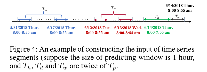
Recent time segments: graph states (features for each node in the graph at a given time) (X_{t_{0} - T_{h} + 1}, X_{t_{0}- T_{h} + 2, \dots, X_{t_{0}}}). In other words, this segment includes the previous T_{h} - 1 times intervals / series. This includes all of the time series within the segment
Daily-periodic segments: a series of intervals of length T_{p}, distributed evenly across T_{d}/T_{p} days of length q (q is the number of samples which are measured per day, so to go to the sample whichw as recorded one day ago at the same time, you need to go to the t_{0} - q + 1 sample)
\begin{align*} & (X_{t_{0} - (T_{d}/T_{p})\cdot q + 1},\dots,X_{t_{0} - (T_{d}/T_{p})\cdot q + T_{p}}, \\ & X_{t_{0} - (T_{d}/T_{p} - 1)\cdot q + 1},\dots,X_{t_{0} - (T_{d}/T_{p})\cdot q + T_{p}}, \\ & X_{t_{0} - (T_{d}/T_{p} - 2)\cdot q + 1},\dots,X_{t_{0} - (T_{d}/T_{p})\cdot q + T_{p}}, \\ & \mskip 2mu \vdots \\ & X_{t_{0} - (1)\cdot q + 1},\dots,X_{t_{0} - (1)\cdot q + T_{p}}\\) \end{align*}
Weekly-periodic segments:
\begin{align*} & (X_{t_{0} - 7\cdot (T_{w}/T_{p})\cdot q + 1},\dots,X_{t_{0} - 7\cdot(T_{w}/T_{p})\cdot q + T_{p}}, \\ & X_{t_{0} - 7\cdot (T_{w}/T_{p} - 1)\cdot q + 1},\dots,X_{t_{0} - 7\cdot(T_{w}/T_{p})\cdot q + T_{p}}, \\ & X_{t_{0} - 7\cdot (T_{w}/T_{p} - 2)\cdot q + 1},\dots,X_{t_{0} - 7\cdot(T_{w}/T_{p})\cdot q + T_{p}}, \\ & \mskip 2mu \vdots \\ & X_{t_{0} - 7\cdot (1)\cdot q + 1},\dots,X_{t_{0} - 7 \cdot (1) q + T_{p}}) \end{align*}
NOTE: Although the ASTGCN models and such can be used through PyTorch geometric (library) The original publication and repository includes support for the standard pytorch functions which may be more straightforward to convert into a CrypTen (CrypTensor) model.
15.2.5 Things I don’t Understand …
- what is the hadammard product?
- the hadamard product is simply the element-wise matrix multiplication of two matrices
- what does it mean to transform the graph convolution setting into the spectral basis, and why is the fourier transform needed to do this? Is it even important for me to answer this question given the setting of the paper itself?
- Probably not important. We will need to understand this theory when doing the writeups, for write now, we just need to know the actual polynomial functions used so we can implement them securely.
15.3 Graph WaveNet
Notes for Graph WaveNet for Deep Spatial-Temporal Graph Modeling Z. Wu (2019)
15.3.1 Contributions
- Methodology uses a stacked dilated 1D convolution in order to get better temporal representations - longer range time series sequences can be processed effectively
- Automatically learns new graph structures - showing hidden spatial dependencies using a “self-adaptive adjacency matrix”
- open source git repository
15.3.2 Methods
- Use a graph convolution layer:
- incorporates graph signal diffusion with K finite steps
- also utilize an adaptive adjacency parameter with learnable embedding parameter dictionaries for nodes in the graph
- Temporal Convolution Layer:
- uses gating mechanisms and dilated causal convolution networks for handling long sequences
- allows for increased receptive field size (expands range while requiring less depth for the network)
- gated TCN layers are stacked in order to improve handling of spatial dependencies at different temporal levels.
15.3.3 Experiments and Evaluation
- experiments conducted on the METR-LA and PEMS-BAY datasets
- baselines
- ARIMA - auto-regressive integrated moving average with Kalman filter
- FC-LSTM - RNN with fully connected LSTM hidden units
- WaveNet - Conv net for sequence data
- DCRNN - diffusion conv recurrent neural nets - combine graph convs. with RNNs in encoder-decoder manner
- GGRU - graph gated recurrent unit network (attention mechanisms used in graph conv.)
- STGCN - spatial-temporal graph convolution network
15.3.4 Questions
- what is an adaptive dependency matrix (as it relates to the learning of the model?)
- receptive field - region of the input image that is used to compute the output of a particular neuron in the feature map. The receptive field is important because it determines the context or the information that the neuron has access to when making a prediction - see medium.com
- what is the receptive field of a convolution?
- What are “stacked dilated 1D convolutions”? See WaveNet for more information on this topic
dilated convolutions - dilated convolutions perform convolutions, but add zeros between the elements of the filter. This expands the receptive field of a given computation by expanding the region of the input covered by a given convolution, but doesn’t increase the number of parameters required to obtain the output. A nice image of this can be seen below:
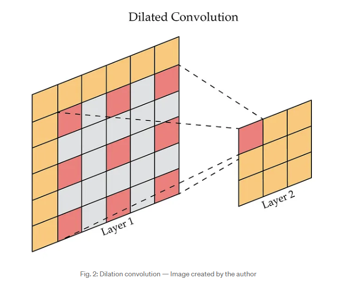
Dilated Convolution Representation
- What does it mean for the adjacency matrix representation of the graph to be “self-adaptive”, and learnable?
- Why is a node’s representation called a node’s “signal” in this work?
- what is a transition matrix?
- I believe this idea originates from this paper: DCNNs
- What is a power series, and how is it applied to a transition matrix?
- What is a TCN layer, let alone a “Gated TCN”? (does this just mean gated temporal convolution?)
- What are gating mechanisms in RNNs, and what are they used for?
- How are graph network structures constructed from the data? See the experimental setup section for more information.
- What is all of this forward-backward adaptive adjacency matrix learning stuff they mention?
- do they train the graph representation of the traffic flow data separately from the actual graph modeling?
15.3.5 Ideas
- integrate alternative gated TCN functions g(\cdot) in order to compare performance in the secure setting. How can this be used as part of a discussion on theory? Is ther even enough time to do this in the project?
- compare the performance of spatio-temporal graph networks along different axes …
- comparative analysis for grpah models - accuracy (MAE/MAPE/RMSE) tradeoffs and running time comparisons (especially for a secure implementation)
15.4 GMAN
These notes are based on the paper GMAN: A Graph Multi-Attention Network for Traffic Prediction published by C. Zheng (2019). The code associated with this model is available through this repository
15.4.1 Contributions
Challenges with Long-Term (a few hours ahead) Predictions
- dynamic spatial correlations - correlations of traffic conditions change significantly over time
- non-linear temporal correlations - traffic conditions at sensors fluctuate drastically and suddenly. Modeling long-term nonlinear relationships is a challenging problem
- sensitivity to error propagation - small errors at each time step propagate, meaning that long-term predictions suffer from accumulated errors.
Innovations and Solutions to Aforementioned Challenges
- Proposed GMAN (Graph Multi-Attention Network)
- features encoder-decoder architecture
- encoder encodes features of the traffic network
- decoder makes predictions based on the features
- encoder and decoder are built on ST-Attention Blocks
- A transform attention layer is added between the encoder and the decoder to convert historical features to generate future representations
- features encoder-decoder architecture
- spatial and temporal attention mechanisms for modeling dynamic spatial and non-linear temporal correlations
- a gated fusion combines information extracted by said mechansims
- transform attention mechanism - converts past traffic features to future representations
- model is evaluated on two real-world traffic datasets (comparative evaluation)
15.4.2 Methods
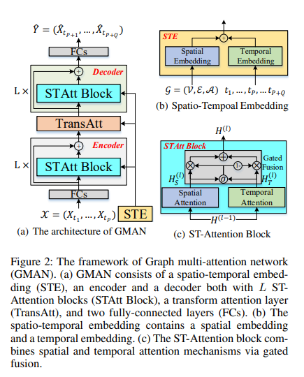
GMAN is constructed from the following components:
- spatio-temporal embedding - incorporates graph structure and time information into the multi-attention mechanism
- encoder
- uses L ST-Attention blocks + residual connections
- ST-Attention has spatial / temporal attention mechansims
- also has gated fusion
- uses L ST-Attention blocks + residual connections
- transform attention layer
- convert encoded features to decoder
- decoder
- also has L ST-Attention blocks and residual connections
Spatio-Temporal Embedding
- spatial embedding is generated from graph data (node2vec approach). this embedding is learned and co-trained with the whole model
- spatial embedding given by e_{v_{i}}^{S} \in \mathbb{R}^{D}, v_{i} \in \mathcal{V}
- temporal embedding is based on a one-hot encoding approach
- T time steps (marked as 1 if the time step is the corresponding one, all zeros for the other T-1 time steps in the vector), and 7 days (using the same embedding approach).
- A two layer fully-connected network transforms this embedding into \mathbb{R}^{D}
- time embeddings are generated for the P past and Q future time steps
- concatentate these time step (per day) and week embeddings to get a single vector embedding of the time (day and the hour*)
- the temporal embedding is given by e_{t_{j}}^{T} \in \mathbb{R}^{D}, t_{j} = t_{1},\dots,t_{P},\dots,t_{P+Q}
- spatial and temporal embeddings are fused to get a spatial-temporal embedding
- spatial-temporal embedding: e_{v_{i},t_{j}} = e_{v_{i}}^{S} + e_{t_{j}}^{T}
ST-Attention Block
There are three elements to each ST-Attention Block
- Spatial Attention
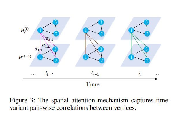
captures correlations between sensors in the road network (dynamic assignment of weights to different vertices [sensors] at different time steps)
a weighted sum of all vertices is given for computing the effect of spatial correlations: hs_{v_{i},t_{j}}^{(l)} = \sum_{v\in \mathcal{V}} \alpha_{v_{i},v} \cdot h_{v,t_{j}}^{(l-1)}
The summation of attention scores is equal to 1: \sum_{v \in \mathcal{V}} \alpha_{v_{i},v} = 1
both graph features, and the graph structure are used in order to learn the attention score \alpha: this logic is derived from the intuition that, for example, congestion on a road may significantly affect the traffic conditions of its adjacent roads.
relevance between vertex v_{i} and v given as: s_{v_{i},v} = \frac{\langle h_{v_{i},t_{j}}^{(l-1)} || e_{v_{i},t_{j}},h_{v,t_{j}}^{(l-1)} || e_{v,t_{j}} \rangle}{\sqrt{2D}}
- || is the concatentation op.
- \langle \cdot, \cdot \rangle is the inner dot product op.
- 2D is the dimension of h_{v_{i},t_{j}}^{(l-1)} || e_{v_{i},t_{j}}
s_{v_{i},v} is normalized via softmax to obtain the attention score \alpha_{v_{i},v} = \frac{\exp(s_{v_{i},v})}{\sum_{v_{r} \in \mathcal{V}} \exp(s_{v_{i}v_{r}})}
the spatial attention is extended to a multi-head attention mechanism (to stabilize learning)
- K parallel attention mechanisms are concatenated together s_{v_{i},v}^{(k)} = \frac{\langle f_{s,1}^{(k)}(h_{v_{i},t_{j}} || e_{v_{i},t_{j}}), f_{s,2}^{(k)}(h_{v,t_{j}}^{(l-1)} || e_{v,t_{j}})\rangle}{\sqrt{d}}
- see the paper for more details on these equations
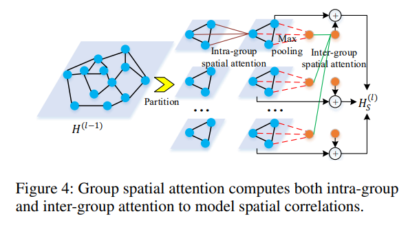
group spatial attention used to address memory and time constraints associated with a high number of vertices (large graph network). Includes intra and inter group attention. N vertices partitioned into G groups
- intra-group attention
- models local spatial correlations among vertices
- inter-group attention
- max pooling is applied to obtain a single representation for each group
- inter-group attention models correlations between different groups - outputs global feature for each group
grouped spatial attention mechanism - intra-group attention
Temporal Attention
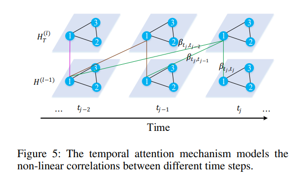
temporal attention non-linear correlations exist between the current and previous traffic states for a given location. (e.g. congestion occuring in morning peak hours may affect traffic conditions for several hours after)
a temporal mechanism is proposed for modeling this correlation
traffic step and time are considered for computing relevance between two time steps (similarity?)
a multi-head attention approach is used:
\begin{align*} & \mu_{t_{t},t}^{(k)} = \frac{\langle f_{t,1}^{(k)}(h_{v_{i},t_{j}}^{(l-1)} || e_{v_{i},t_{j}}),f_{t,2}^{(k)}(h_{v_{i},t}^{(l-1)} || e_{v_{i},t})\rangle}{\sqrt{d}} \\ & \beta_{t_{j},t}^{(k)} = \frac{\exp(u_{t_{j},t}^{(k)})}{\sum_{t_{r} \in \mathcal{N}_{t_{j}} \exp(u_{t_{j},t_{r}}^{(k)})}} \end{align*}
- u_{t_{j},t}^{(k)} - relevance between time step t_{j} and t
- \beta_{t_{j},t}^{(k)} - attention score in the k\text{-th} head (the importance of time step t to t_{j})
- \mathcal{N}_{t_{j}} - set of time steps before t_{j}
hidden state of vertex v_{i} at time step t_{j} given by: ht_{v_{i},t_{j}}^{(l)} = ||_{k=1}^{K} \left\{\sum_{t\in \mathcal{N}_{t_{j}}}\beta_{t_{j},t}^{(k)}\cdot f_{t,3}^{(k)}(h_{v_{i},t}^{(l-1)})\right\}
- f_{t,3}^{(k)}, f_{t,2}^{(k)}, and f_{t_{1}^{(k)}} - learnable non-linear projections
Gated Fusion
traffic is dependent upon previous traffic flows (temporal) and the traffic at other roads (spatial)
gated fusion fuses the temporal and spatial representations
these representations are fused in the decoder as:
\begin{align*} & H^{(l)} = z \odot H_{s}^{(l)} + (1-z) \odot H_{T}^{(l)} \\ & z = \sigma(H_{S}^{(l)} + (1-z)\odot H_{T}^{(l)}) \end{align*}
- H_{S}^{(l)} and H_{T}^{(l)} are the spatial and temporal outputs of the network at the l\text{-th} block
Transform Attention
![]()
- A transform attention layer is added between the encoder and decoder
- it determines relationship between past time steps and future representations - passed as input to the decoder
- relevance between prediction time step t_{j} and historical time step t given by spatio-temporal embedding \lambda_{t_{j},t}^{(k)}
- \lambda_{t_{j},t}^{(k)} is used to calculate the attention score \gamma_{t_{j},t}^{(k)}
- relevant features are selected from across P time steps and transmitted to the decoder
Encoder-Decoder
- historical observations are transformed into the vertex embedding space: X \rightarrow H^{(0)}
- the embedding is passed to the encoder with L ST-Attention blocks: H^{(L)} is output
- transformer attention layer converts encoded features H^{(L)} to future representation H^{(L+1)}
- decoder stacks L ST-Attention blocks on H^{(L+1)} to get H^{(2L + 1)}
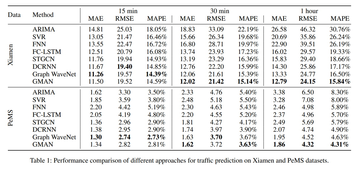
15.4.3 Evaluation
- datasets:
- Xiamen
- PeMSBay
- compare against the following methods:
- ARIMA
- SVR
- FNN
- FC-LSTM
- DCRNN
- Graph WaveNet
- preprocessing:
- time steps denote 5 minute intervals
- data normalized by z-score method
- 70%, 10%, 20% - train, val, test data split
- if the distance between two sensors in the road network is beneath some threshold, then an edge is added to the graph connecting the two nodes in question. Otherwise, no edge is added to connect two points directly.
15.4.5 Questions
- are the attention mechanisms more computationally efficient in smpc than other modes or no? this might be the most interesting question to answer.
15.5 STSGCN
Notes based on the paper Spatial-Temporal Synchronous Graph Convolutional Networks: A New Framework for Spatial-Temporal Network Data Forecasting. The associated GitHub repository is linked here
15.5.1 Contributions
Prior to the introduction of STSGCN, other works had separately considered the effect of spatial and temporal correlations in traffic flow patterns. However, none had successfully incorporated the spatial-temporal (interacting) correlations and patterns. This contribution, or attempted contribution, is similar to that of ST-SSL (Section 15.7). However, the way in which they achieve this effect is slightly different:
- they propose a spatial-temporal graph convolutional module to directly capture localized spatial-temporal correlations instead of using separate modules separately (to indirectly monitor this correlation)
- capture heterogeneity in long-range spatial-temporal graphs
- multiple modules are deployed on each time period (spatial-temporal correlations are captured on each localized spatial-temporal graph)
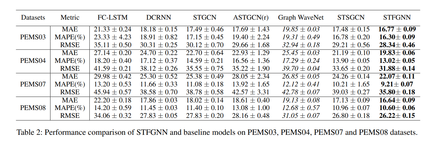
- experiments for four dataset (PeMS-03,04,07,08) to validate model performance.
15.5.2 Methods
An overview of the network architecture is given in the graphic below:
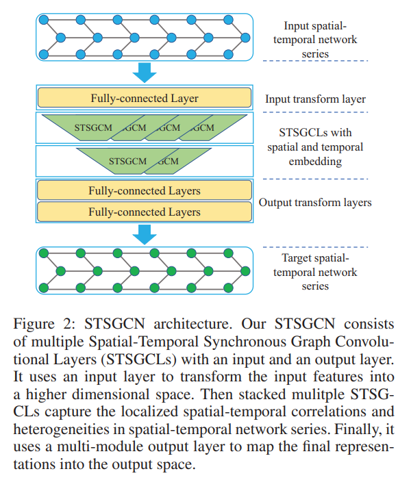
There are three core points underlying the construction of STSGCN:
- each node is connected to itself at the previous and next time steps to construct a localized spatial-temporal graph
- a spatial-temporal synchronous graph convolutional module is developed to capture the localized spatial-temporal correlations
- deploy multiple modules to model heterogeneities in spatial-temporal network series.
Localized Spatial-Temporal Graph Construction
- Capture impact of each node on its neighbors belonging to the current and adjacent time steps
- connect all nodes with themselves at adjacent time steps
- get localized spatial-temporal graph as result
- A \in \mathbb{R}^{N \times N} - adjacency matrix of spatial graph
- A' \in \mathbb{R}^{3N \times 3N} - adjacency matrix of localized spatial-temporal graph
- the diagonal of A' are the adjacency matrices of three contiguous time steps
- two sides of diagonal indicate connectivity of each node to itself (belonging to adjacent time steps)
Spatial-Temporal Embeddings
- The base initialization of the Spatial-Temporal graph does not distinguish between nodes at different time steps
- spatial and temporal embedding matrices are trained, and added to the temporal network series in order to obtain new representations for the network series.
Spatial-Temporal Synchronous Graph Convolutional Module
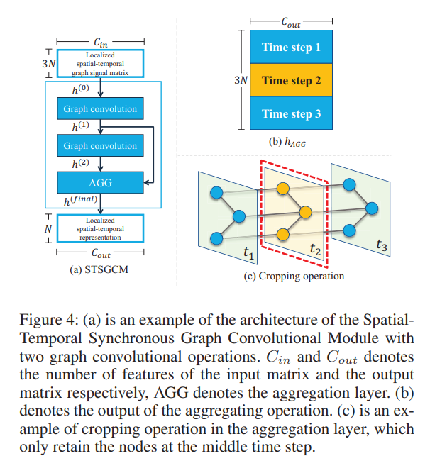
- STSGCM (module) consists of:
- a series of graph convolution operators:
GCN(h^{(l-1)}) = h^{(l)} = \sigma(A'h^{(l-1)}W + b) \in \mathbb{R}^{3N \times C'}
- \sigma denotes the GLU activation function utilized
- Graph convolutional layer is formulated as:
h^{(l)} = (A'h^{(l-1)}W_{1} + b_{1}) \odot sigmoid(A'h^{(l-1)}W_{2} + b_{2})
- the gated linear unit controls which node’s information is passed to the next layer
- graph conv op. defined over vertice domain: does not need to compute graph laplacian
- self-loops added to eac node in the localized spatial-temporal graph so that nodes can take in information about themselves when aggregating features
- a series of graph convolution operators are stacked to increase the receptive field
- outputs of the graph convolution layers are fed to the aggregation layer (compacts outputs)
- involves cropping and aggregating
- aggregation operation: max pooling
- cropping operation: removes features of nodes at previous and next time steps, so only the middle time step remains. Since the graph conv. operations have already aggregated information from other nodes (in the spatial-temporal graph) to these nodes by this point, the remaining nodes still store spatial-temporal information relevant to the other time steps.
- a series of graph convolution operators:
GCN(h^{(l-1)}) = h^{(l)} = \sigma(A'h^{(l-1)}W + b) \in \mathbb{R}^{3N \times C'}
STSGCL - Using Multiple Modules to model Heterogeneities
Note: STSGCL stands for Spatial-Temporal Synchronous Graph Convolutional Layer
- a sliding window is used to cut out different periods (time)
- spatial-temporal data is heterogeneous, so it is better to use several STSGCMs to model each of the spatial-termporal corrleations in the localized graph
- First, spatial-temporal embeddings are added to the input (as discussed above)
- Then, the sliding window divides the input into T-2 spatial-temporal network series (T - the number of time steps in the input series X \in \mathbb{R}^{T\times N\times C})
- T-2 STSGCM modules are used on the T-2 spatial-temporal network series - each of the spatial-temporal network series has three time steps …
- outputs are concatenated togehter into a single matrix:
M = [M_{1},M_{2},\dots,M_{T-2}] \in \mathbb{R}^{(T-2) \times N \times C_{out}}
- M_{i} \in \mathbb{R}^{N \times C_{out}} - the outputs of the i\text{th} STSGCM
- multiple STSGCLs are stacked (as shown in the figure below) to build a hierarchical model.
Additional Components
- Masking matrix:
- a weight mask matrix W_{mask} is trained to adjust the aggregation weights to improve the aggregation step of the STSGCM A'_{adjusted} = W_{mask} \otimes A' \in \mathbb{R}^{3N \times 3N}
- Input Layer:
- FC layer added at top of network to transform input into a higher dimensional space
- Output Layer:
- Two FC layers are used to geerate final predictions (input is the output of the last STSGCL). \hat{y}^{(i)} = ReLU\left(X^{T}W_{1}^{(i)} + b_{1}^{(i)}\right)\cdot W_{2}^{(i)} + b_{2}^{(i)} Here, \hat{y}^{(i)} indicates the prediction in time step i.
- predictions \hat{y}^{(1)}, \hat{y}^{(2)}, \dots, \hat{y}^{(T)} are concatenated to obtain the overall output
- Training:
- The Huber Loss function is used for optimization
- has a \delta parameter to control for range of squared errror loss (reduces sensitivity of loss to outliers)
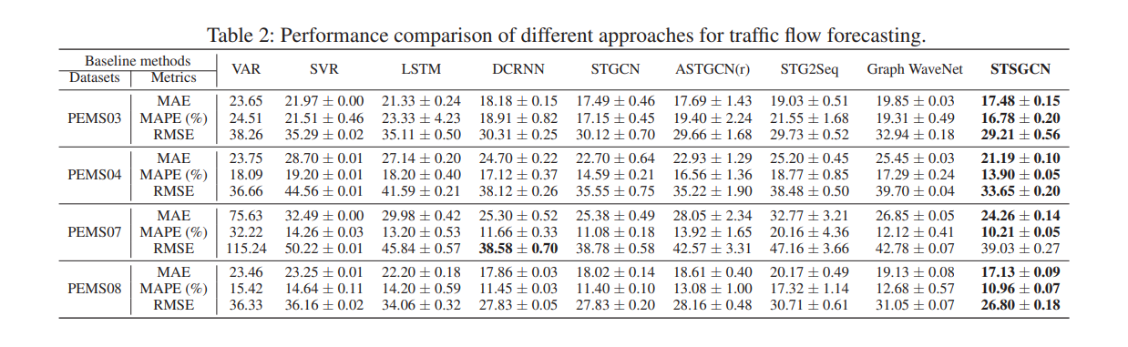
15.5.3 Evaluation
- Datasets
- use four datasets:
- PEMS03
- PEMS04
- PEMS07
- PEMS08
- flow data is aggregated to 5 minute intervals
- the past hour of data points are used to predict the next hour’s behavior
- If two sensors are on the same road, they are considered to be connected in the spatial network (add an edge)
- features of the graph are standardized by centering and scaling
- use four datasets:
- Baselines
- VAR (vector auto-regression)
- SVR
- LSTM
- STGCN
- ASTGCN(r)
- STG2Seq
- Graph WaveNet
- Results
15.5.4 Comments
- I don’t find this work particularly inspiring. It might be interesting to evaluate, purely as a point of comparison to other models. It’s not clear to me that the architecture of this model is any simpler, or more efficient than any of the other grpah models which were presented as an alternative.
15.6 STFGNN
Notes are based on the paper Spatial-Temporal Fusion Graph Neural Networks for Traffic Flow Forecasting published in M. Li (2021) for AAAI2021. The GitHub repository for their model is available here
15.6.1 Contributions
- Prior limitations of spatial-temporal traffic forecasting models
- lack of informative graph construction (un-represented correlations between distant nodes). E.g.) at rush hour, roads near office buildings will encounter traffic jams in the same period. Most graph constructions only account for spatial information, but ignore temporal similarity between nodes
- studies of spatial-temporal data forecasting, ineffective at capturing dependencies between local / global correlations
- RNN / LSTM methods - slow and suffer vanishing / exploding gradient
- CNN - require stacking of many layers to capture global correlations (for long sequences). local information is lost when dilation rate increases …
Novelty and Innovations:
- new, data-driven method for graph construction (temporal graph is learned based on similarities between time series) - this method is motivated by the dynamic time warping problem/algorithm
- note: dynamic time warping is an algorithm used for measuring the similarity between two time series, X = (x_{1},x_{2},\dots,x_{n}) and Y = (y_{1},y_{2},\dots,y_{m}). It uses a dynaic programming approach in order to iteratively construct the optimal distance matrix M_{n \times m}. The core of the problem is solving the warping curve (matchup of series points x_{i} and y_{j}) \Omega = (\omega_{1},\omega_{2},\dots,\omega_{\lambda}), \mskip 1mu \max(n,m) \le \lambda \le n + m elements \omega_{\lambda} = (i,j) is the matchup of x_{i} and y_{j}
- gated dilated convolution module introduced (large dilation rate captures long-range sequences) - how does it avoid losing local correlations?
Secure Setting:
- use plaintext, learned models for constructing the graph, submit the learned graph to the private model for inference on future time steps i.e., the user preprocesses their data and then sends it to the server.
15.6.2 Methods
Basic Overview of STFGNN
A visual representation of the STFGNN architecture is given below:
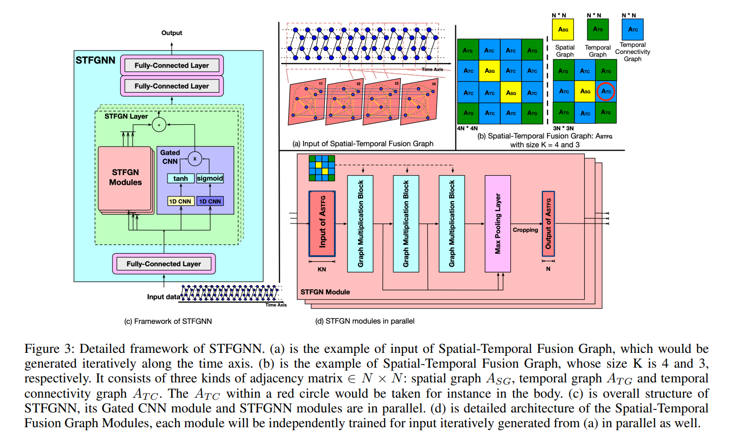
\begin{align*} & \text{input layer} \rightarrow \text{FCC} + ReLU \\ & \downarrow \\ & \text{stacked spatial-temporal fusion graph neural layers} \\ & \mskip 2mu \text{STFGN Modules} + \text{Gated CNN} \\ & \downarrow \\ & \text{output layer} \rightarrow 2\times\text{FCC} + ReLU \end{align*}
Temporal Graph Construction
A visual representation of the dynamic time warping algorithm used to construct spatial-temporal fusion graphs:
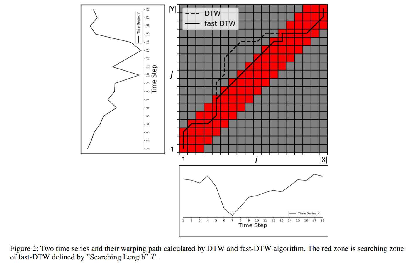
- light-DTW is used to generate the temporal graph based on the similarity of two time-series. Bascicaly, the search space of the algorithm is limited in order to make its use feasible in larger scale time-series data
- the warping path between two time-series is restricted by the bound T
- three elements to the spatial-temporal fusion graph A_{STFG} \in \mathbb{R}^{KN \times KN}:
- A_{TG} - the temporal graph - is weighted and givn by alg 1.
- A_{TC} - elements are nonzero if and only if previous and next time steps are the same node
- A_{SG} - the spatial graph component - this is given by the dataset itself.
Spatial-Temporal Fusion Graph Neural Module (STFGN Modules)
- spatial-temporal dependencies extracted via several matrix multiplciations over the fusion graph A_{STFG}. residual connections and max pooling are incorporated as well (training efficiency, etc.)
- matrix multiplication replaces less efficient laplacian spectral graph convolutions
Graph Multiplication Blocks
- utilize a gating mechanism (like LSTM/RNN)
- GLU is used for generalization in graph multiplciations by its nonlinear activation
- mathematical formulation:
h^{l+1} = (A_{STFG}h^{l}W_{1} +b_{1}) \odot \sigma(A_{STFG}h^{l}W_{2} + b_{2})
- h^{l} is the l-th hidden state of the STFGN module
- \odot is element-wise multiplication (hadamard product)
Pooling and Cropping
- outputs / hidden states for each graph multiplication block is concatenated and passed through max pooling. The output is then cropped
Multiple STFGN modules process the input independently (in parallel), and their outputs are concatenated together, along with the output of the gated CNN layer. This concatenated output is passed to the next STFGN layer (STGFN modules and a gated CNN make up each STFGN layer)
Gated Convolution (Gated CNN)
- dilated convolutions are used with a large dilation rate
- mathematical formulation: Y = \phi(\Theta_{1} * X + a) \odot \sigma(\Theta_{2} * X + b)
Training
The Huber loss is used as the loss function for training the model. A parameter \delta is used to control sensitivity of the squared error loss.
15.6.3 Evaluation
- datasets:
- PEMS03
- PEMS04
- PEMS07
- PEMS08
- data collected from the Caltrans Performance Measurement system and aggregated into 5-minute windows (288 points in the traffic flow for one day)
- spatial adjacency networks are constructed by the actual road network based on distance
- z-score normalization is used to standardize inputs
- compare against the following methods
- FC-LSTM
- DCRNN
- STGCN
- ASTGCN(r)
- GraphWaveNet
- STSGCN
15.6.4 Comments and Thoughts
- This model may be stronger for smpc applications since it is lightweight. Namely it doesn’t require spectral graph convolutions which are time consuming. The size and depth of the architecture can also be compared with other models. Moreover, some of the graph formulation and preprocessing is done beforehand, which might make the inference stage more efficient as well.
15.6.5 Questions
- How does the DTW algorithm work?
- How is the graph analyzed when formulated as they do (the concatenation of a series of subgraphs represented as a single matrix)
15.7 ST-SSL
Use this as a benchmark for everything else. We want to figure out what were the other top models to evaluate. This paper is very recent, and it comes out of a top conference (AAAI). Notes for this section based on ST-SSL by Ji et al. J. Ji (2023). The GitHub repository for this model is available here
This work is the current state of the art in traffic flow forecasting and prediction tasks. They evaluate their models on the NYBike1 and other more challenging datasets, instead of the Pems datasets as was the case with most prior works.
15.7.1 Contributions
ST-SSL was designed to address two key limitations of existing methods for traffic flow prediction:
- lack of modeling spatial heterogeneity exhibited with skewed traffic distributions across different regions
- different regions (urban versus residential) can have very different traffic flow from one another
- leads to biasing towards regions with higher traffic volume
- prior solutions [Pan et al. 2019b; Bai et al. 2020] required large parameter sizes, and were computationally expensive - meaning that they were unable to handle larger datasets
- other solutions consider differences across regional traffic distributions, but this requires considerable hand engineering, making it difficult to generalize such solutions to other problems and datasets.
- Current traffic prediction methods model temporal dynamics using a shared parameter space for all time periods - does not preserve temporal heterogeneity.
- e.g.) the difference between morning and night, holidays, workdays, etc.
Solutions:
- spatial-temporal pattern capture:
- ST-SSL is a graph neural network - uses temporal and spatial convolutions for information aggregation.
- Spatial heterogeneity capture:
- self-supervised supervised learning paradigm for augmenting traffic flow graph (data-level and structure-level) - adapts well to heterogeneous regions and traffic distributions
- Temporal heterogeneity:
- auxiliiary self-supervision with clustering
- indicates diverse spatial patterns across regions
- ST-SSL maintains dedicated representations of temporal traffic dynamics with a self-supervised learning paradigm
15.7.2 Model Overview and Novelty
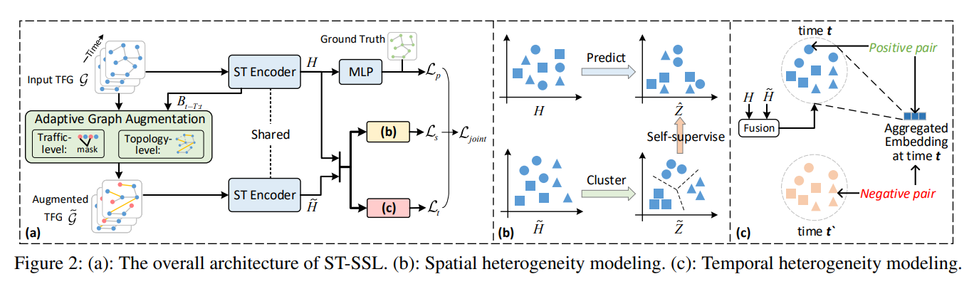
Spatio-Temporal Encoder (ST Encoder)
- jointly preserves the spatio-temporal contextual information over the traffic flow graph - enables modeling of sequential patterns of traffic data (across different time steps) and the geographic correlations among spatial regions
- temporal convolution and graph convolution is backbone for spatial-temporal relational representation
- Temporal convolutions:
- 1D causal convolution along the tiem dimension + gated mechanism
- (B_{t-T_{out}},\dots,B_{t}) = TC(X_{t-T},\dots,X_{t}) - B_{t}\in \mathbb{R}^{N \times N} denotes the region embedding for r_{n}
- D - embedding dimensionality
- T_{out} - length of embedding sequence after conv. operations in TC encoder
- Spatial Convolutions:
- E_{t} = SC(B_{t}, A)
- A - region adjancency matrix of g
- results in refined embeddings (E_{t - T_{out}},\dots,E_{t})
STEncoderhas a sandwhich block structure:TC -> SC -> TC- output: sequence of embedding matrices - (H_{t-T'},\dots,H_{t})
Adaptive Graph Augmentation
- Adaptive augmentation is performed on (B_{t-T_{out}},\dots,B_{t}) - the region embeddings for timesteps t-T_{out} to t.
- There are two modes of graph augmentation used: (1) graph topology-level augmentation and (2) traffic-level data augmentation
Measuring region-wise heterogeneity
- A given region, r_{n} has an embedding sequence (b_{t-T_{out},n},\dots,b_{t,n}). The aggregated representation of region r_{n} across time steps based on aggregation weight p_{\tau,n}
u_{n} = \sum_{r=t-T}^{t} p_{\tau,n} \cdot b_{\tau,n}, \text{ where } p_{\tau,n}=b_{\tau,n}^{T}\cdot w_{0}
- The graph augmentation step is important since it allows for identifying heterogeneity across the different regions both spatially and temporally. The degree of heterogeneity between any two regions (the traffic distribution difference over time) is given by:
q_{m,n} = \frac{u_{m}^{T}u_{n}}{||u_{m}||||u_{n}||}
- Larger values of q_{m,n} indicate a greater traffic pattern dependency (stronger correlation) between regions r_{m} and r_{n}. The observed degree of heterogeneity guides the augmentation of graph topology and traffic data alike. High values of q_{m,n} also indicate a low level of heterogeneity between the two regions.
Traffic-Level Augmentation
- X_{t-T:t} is the constructed traffic tensor. An augmentation operator is designed to operate over this tensor and adapt to the time-correlated traffic patterns for each region.
- the augmentation operator masks less relevant traffic volume at the \tau\text{th} time step of region r_{n} against noise perturbation
- this is given by a derived masking probability p_{\tau,n} \sim \text{Bern}(1-p_{\tau,n})
- higher p_{\tau,n} \rightarrow region r_{n} has traffic volume x_{\tau,n} at the \tau-th timestep which will more likely be masekd due to its lower relevance for traffic regularities of region r_{n}
- augmented data: \tilde{X}_{t-T:t}
Graph Topology-Level Augmentation
- for any two adjacent regions, r_{m} and r_{n}, if their respective value of q_{m,n} is low, the edge connecting the two regions will be masked.
- mask probability: p_{m,n} \sim \text{Bern}(q_{m,n})
- for non-adjacent regions, r_{m} and r_{n}, if there is low heterogeneity (high q_{m,n}) for the two nodes, an edge will be added based on the masking probability p_{m,n}. i.e. the probability of adding an edge is given by q_{m,n}^{y}(1-q_{m,n})^{1-y}, where y=0,1 (0 indicates the edge will not be added, and 1 indicates it will)
- graph topology augmentations help to debias traffic volume input and denoise the graph structure
SSL for Spatial Heterogeneity Modeling (a)
- soft clustering is used to group different regions into K latent categories
- generate K cluster embeddings \{c_{1},\dots,c_{K}\} (indexed by k)
- clustering is performed as
\tilde{z}_{n,k} = c_{k}^{T}\tilde{h}_{n}
- \tilde{z}_{n,k} is a measure of the estimated relevance / connection between
- \tilde{h_{n}} - the region embedding of a region r_{n} from the augmented graph
- c_{k} embedding on the k\text{th} cluster.
- The cluster assignment is generated based on this score
- the self-supervised augmented task is optimized for the following:
\ell(h_{n}, \tilde{z}_{n}) = -\sum_{k}\tilde{z}_{n,k}\log \frac{\exp(\hat{z}_{n,k}/\gamma)}{\sum_{j}\exp(\hat{z}_{n,j}/\gamma)}
- \gamma - temperature parameter to control smoothing of softmax output
- overall self-supervised objective function:
L_{s} = \sum_{n=1}^{N}\ell(h_{n},\tilde{z}_{n})
- this caues the region embedding h_{n} to be reflective of spatial heterogeneity within the global urban space
Distribution Regularization
- two main issues to address with this formulation
- Issue 1: because of how the cluster assignment matrix is generated, there is no guarantee that the sum of the cluster assignment will be 1 for each region.
- Issue 2: we want to avoid the trivial solution that all regions are assigned to the same cluster.
- solution 1: the principle of maximum entropy is used to encourage regions to be equally partitioned by clusters
SSL for Temporal Heterogeneity Modeling (b)
Temporal heterogeneity is modeled in four steps:
- Step 1: fuse the original and augmented encoded time-aware region embeddings v_{t,n} = w_{1} \odot h_{t,n} + w_{2} \odot \tilde{h}_{t,n}
- Step 2: aggregate the region level embeddings to generate a city-level embedding representation at time step t: s_{t} = \sigma\left(\frac{1}{N}\sum_{n=1}^{N}v_{t,n}\right)
- Step 3: Represent pairs of region and city level embeddings as positive if the region and city-level embeddings are from the same time step, and negative if the embeddings are from different time steps
- Step 4: Optimize the cross-entropy losss:
L_{t} = -\left(-\sum_{n=1}^{N}\log g(v_{t,n},s_{t}) + \sum_{n=1}^{N}\log(1-g(v_{t',n},s_{t}))\right)
- t and t' denote two different time steps
- g is the criterion function g(v_{t,n},s_{t}) = \sigma(v_{t,n}W_{3}s_{t})
- W_{3} \in \mathbb{R}^{N \times N} - a learnable transformation matrix
The effect of this temporal heterogeneity modeling is two-fold:
- labeling of pairs with the same time-step encourages the consistency of time-specific citywide traffic trends
- labeling pairs from different time steps as negative captures the temporal heterogeneity across different time steps
15.8 STPGCN
PyTorch repository for this model The Notes from this section are based on the paper: “Spatial-Temporal Position-Aware Graph Convolution Networks for Traffic Flow Forecasting” Y. Zhao (2023)
15.8.1 Contributions
- introduce a spatial-temporal graph representation - models (1) spatial, (2) temporal, and (3) joint spatial-temporal correlations
- develop a position embedding module - encodes spatial-temporal position factors and relation inference module - learn dynamic spatial temporal edge weights
- the authors try to incorporate node-specific patterns and information (from historical data) to improve prediction accuracy at each node. They propose a graph operator,
STPGConvfor this purpose, as it captures a wide range of spatial, temporal, and joint spatial-temporal correlations - the network computes spatial-temporal relations in using a pure graph convolution approach. no external temporal components are required, which improves overall efficiency (at least according to their experimental results)
- design an L-layer network based on the
STPGConvoperation- includes skip connections
- gated selection modules
- these additions help to overcome problem of vanishing gradient and feature over-smoothing
- concatenate features generated by multiple network layers to get an MLP predictor that directly predicts multi-step traffic flows
- typical layer count is L=3. possesses fewer parameters, is computationally efficient
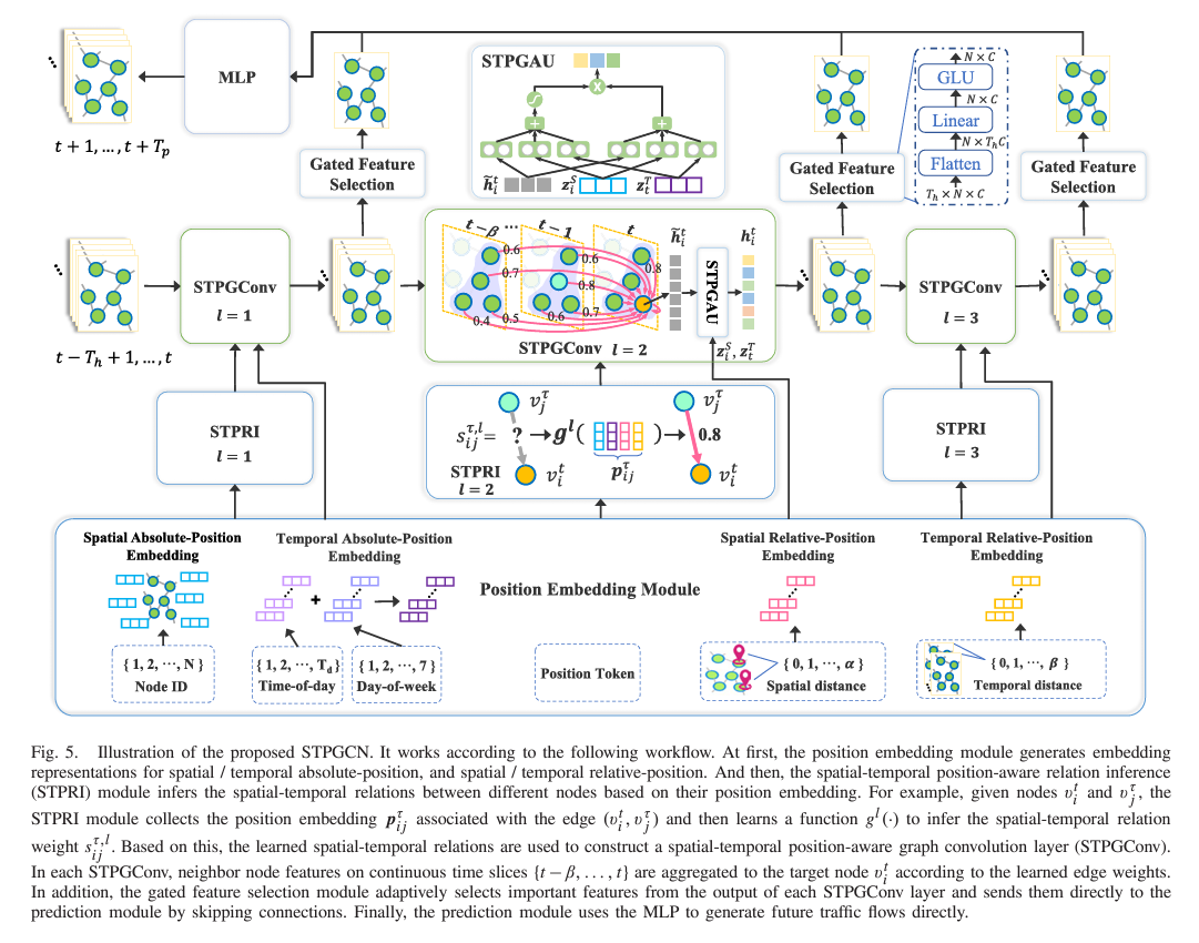
15.8.2 Methods
Zhao et al. propose a novel model and graph convolution architecture for predicting traffic flows based on spatio-temporal information:
Step 1: formulate the graph
- the spatio-temporal graph is represented as a series of \beta time steps t,t-1,\dots,t-\beta where each time step is represented by a graph \hat{A} \in \mathbb{R}^{N \times N}. \begin{align*} A_{STP} = \begin{array}{ccccccc} & & t & t-1 & \dots & t - \beta & \\
t & [ & \hat{A} & \hat{A} & \dots & \hat{A} & ] \end{array}\end{align*}
\hat{A} is an \alpha-hop adjacency matrix of the road network: a picture of these hops can be seen below:
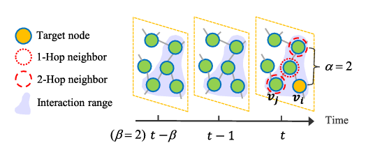
spatio-temporal connection range each element of \hat{A}, the adjacency matrix, is given as follows: \hat{A}_{ij} = \begin{cases} 1 & \text{if SDist}(v_{i}, v_{j}) \le \alpha, \\ 0 & \text{if the shortest path between } v_{i} \text{ and } v_{j} > \alpha \end{cases} in other words, if the shortest path between any two nodes in the spatial direction is of a distance less than \alpha, then there is an \alpha-hop edge which connects the two nodes - hence a 1 fills that connection label in the matrix \hat{A} Graph Edge Weights
Step 2: Set edge weights for the unweighted graph
- spatial and temporal absolute-position embeddings
- spatial embeddings are defined - represent the absolute position of a given vector z^{S} = [z_{1}^{S}, z_{2}^{S}, \dots, z_{N}^{S}] \in \mathbb{R}^{N \times d}
- temporal embeddings are defined similarly z^{S} = [z_{1}^{T}, z_{2}^{T}, \dots, z_{N}^{T}] \in \mathbb{R}^{T_{d} \times d} where Z_{t}^{T} = z_{m}^{D} + z_{n}^{W}.
- z_{m}^{D} - the temporal position embedding for the day - \{1,2,\dots,T_{d}\}
- z_{n}^{W} - the temporal position embedding for the week- \{1,2,\dots,7\}
- these are summed together to obtain the temporal position embedding
- spatial and temporal relative-position embeddings
- these embeddings encode the relative distances between two nodes
- relative spatial and temporal distances between two nodes given as the shortest paths between them across each dimension: \begin{align*} & \text{SDist}(\cdot,\cdot) \rightarrow a \in \{0,1,\dots,\alpha\} \\ & \text{TDist}(\cdot,\cdot) \rightarrow b \in \{0,1,\dots,\beta\} \end{align*}
- the temporal distance can be no more than \beta, and the spatial distance can be no greater than \alpha.
- when a=0, the two nodes are in the same position (spatially)
- when b=0, the two nodes are in the same time slice
- distance values, a and b -> discrete label tokens and generate trainable embedding vectors
- Spatial and temporal relative-position embedding vectors generated as: \begin{align*} & Z^{SD} = [z_{0}^{SD}, z_{1}^{SD}, z_{2}^{SD},\dots,z_{\alpha}^{SD}] \in \mathbb{R}^{(\alpha + 1) \times d} \\ & Z^{TD} = [z_{0}^{TD}, z_{1}^{TD}, z_{2}^{SD}, \dots, z_{\beta}^{TD}] \in \mathbb{R}^{(\beta + 1) \times d} \end{align*}
- it’s not obvious to me what the d symbolizes …
- spatial-temporal position-aware relation inference
- this module takes the embeddings generated for each node, and uses them to map the value of weights for each edge in the graph (dynamic - can change for different time steps)
- you have a node v_{i}^{t} with candidate neighbors v_{j}^{\tau} in the interaction range i,j \in \{1,2,\dots,N\}, t \in \{1,2,\dots,T_{h}\}, \tau \in \{t-\beta, t-\beta+1,\dots,t\} and t-\beta > 0
- S^{t} = \{s_{ij}^{\tau}|i,j=1,\dots,N;\tau=t-\beta,\dots,t\}\in \mathbb{R}^{N \times (\beta + 1)N}
- denote dynamic weights for all spatio-temporla edges
- A^{t}_{STP} = S^{t} \odot A_{STP} - element-wise multiplication of the edge weights by the adjacency matrix.
- each element of S^{t}, s_{ij}^{\tau} is given by s_{ij}^{\tau} = \begin{cases} g(p_{ij}^{\tau}) & \text{if SDist}(v_{i}^{t}, v_{j}^{\tau}) \le \alpha \\ 0 & \text{otherwise} \end{cases}
- p_{ij}^{\tau} is the position feature vector
- p_{ij}^{\tau} = [z_{i}^{S} || z_{j}^{S} || z_{t}^{T} || z_{\tau}^{T} || z_{a}^{SD} || z_{b}^{SD}] \in \mathbb{R}^{6d}
- z_{i}^{S}, z_{t}^{T} - spatial / temporal position info of node v_{i}^{t}
- z_{j}^{S}, z_{\tau}^{T} - spatial / temporal position information of node v_{j}^{\tau}
- z_{a}^{SD}, z_{b}^{TD} - spatial / temporal distance between v_{i}^{t} and v_{j}^{\tau}
- g(\cdot) is a learnable Gaussian kernel for mapping weights from embedding vector inputs
- g(p_{ij}^{\tau}) = \exp\left(-\frac{1}{2}(p_{ij}^{\tau} - \mu)^{T}\sum^{-1}(p_{ij}^{\tau} - \mu)\right)
- \sum = \text{diag}(\sigma) - trainable diagonal covariance matrix
- \mu \in \mathbb{R}^{6d} - trainable mean vector
- \sigma \in \mathbb{R}^{6d} - trainable variance vector
Step 3: Perform Spatial-Temporal Position-Aware Graph Convolution
- joint spatial-temporal node feature aggregator STPGConv
- in each
STPGConvlayer, the dynamic spatial-temporal edge weights are generated based on the position embedding p_{ij}^{\tau} - weight summation function is constructed: \begin{align*}
& \tilde{H}^{t,l} = \phi_{stpgcn}(A_{STP}^{t,l}, \hat{H}^{t,l-1}) = S^{t,l}\hat{H}^{t,l-1} \\
& \text{where } \hat{H}^{t,l-1} = [H^{t,l-1};\dots;H^{t-\beta,l-1}] \in \mathbb{R}^{(\beta+1)N \times C}
\end{align*}
- represent node features output from layer l-1 on \beta + 1 time slices
- The discrete STPGCN operation is given by \begin{align*}
\tilde{h}_{i}^{t,l} &= \phi_{stpgcn}(s_{ij}^{\tau,l}, h_{j}^{\tau,l-1}) \\
&= \sum_{j=1}^{N}\sum_{\tau=t-\beta}^{t} s_{ij}^{\tau,l}\cdot h_{j}^{\tau,l-1}
\end{align*}
- s_{ij}^{\tau,l} - weight of edge connecting nodes v_{i}^{t} and v_{j}^{\tau} (in the l\text{th} layer)
- h_{j}^{\tau,l-1} - the features of node v_{j}^{\tau} from the previous layer
- A linear layer is applied on \tilde{h}_{i}^{t,l} to obtain the traffic flow signal of node v_{j}^{\tau}, h_{j}^{\tau,0} h_{j}^{\tau,0} = W^{0} \cdot x_{j}^{\tau} + b^{0} h_{i}^{t,l} = \Psi(W^{l} \cdot \tilde{h}_{i}^{t,l} + b^{l})
- \Psi - the activation function
- in each
- spatial-temporal position-aware gated activation unit STPGAU
- gating activation units are used to maintain the feature patterns across different time steps for individual nodes.
- formulation: \begin{align*}
h_{i}^{t,l} &= \text{STPGAU}(\tilde{h}_{i}^{t,l}, z_{i}^{S}, z_{t}^{T}) \\
&= (W_{1}^{l} \cdot \tilde{h}_{i}^{t,l} + W_{2}^{l} \cdot z_{i}^{S} + W_{3}^{l}\cdot z_{t}^{T} + b_{1}^{l}) \\
&\mskip 2mu \odot \delta (W_{4}^{l} \cdot \tilde{h}_{i}^{t,l} + W_{5}^{l} \cdot z_{i}^{S} + W_{6}^{l} \cdot z_{t}^{T} + b_{2}^{l})
\end{align*}
- the spatial and temporal embedding vectors are incorporated into the sums in order to maintain the individual patterns and post-tune the output of the
STPGConvlayer to generate node-specific pattern features
- the spatial and temporal embedding vectors are incorporated into the sums in order to maintain the individual patterns and post-tune the output of the
Step 4: Gated Feature Selection and Skip Connections
- avoid gradient vanishing problem by sending outputs of each
STPGConvlayer to the output via skip connections - a gated feature selection module is used to select (adaptively) important features from multiple layers for the final prediction to avoid the over-smoothing problem
Step 5: Make Predictions
- an MLP is used to generate future multi-step results directly - this is done using inputs from the L layers of features generated by the network U = \hat{H}^{1} || \cdots || \hat{H}^{L}
- thes inputs are fed to the MLP to make preidctions
15.8.3 Evaluation
15.8.4 Questions
- I still don’t know what “Gated Activation Units” are
16 Trajectory-Based Traffic Forecasting
16.1 ST-ResNet
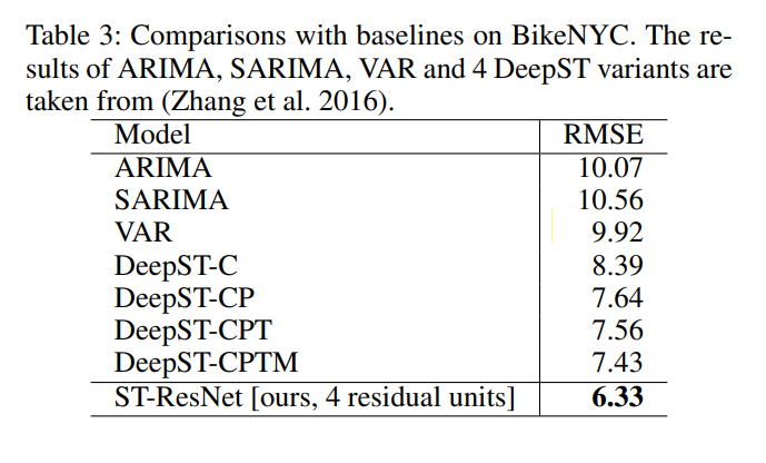
These notes are based on the paper Deep Spatio-Temporal Residual Networks for Citywide Crowd Flows Prediction published by J. Zhang (2017). The original open-source repository is available here. An updated repository with preprocessing optimizations is available here
16.1.1 Contributions
- present ST-ResNet: convolution-based residual networks for modeling local and distance spatial dependencies between any two regions of a city
- temporal properties grouped into three categories - each is modeled by a separate residual network
- temporal closeness
- period
- trend
- external factors (weather, holiday info, etc.) are modeled by an additional resnet
- outputs of the resnets are aggregated (with diff. weights for branches / regions)
- evaluate the model on
- Beijing Taxicabs
- NYC bike trajectory data
16.1.2 Methods
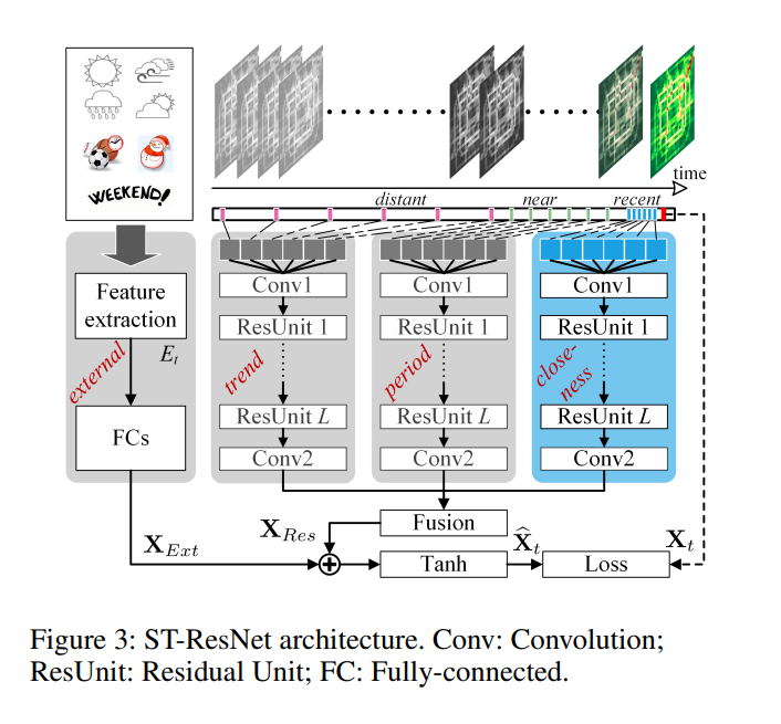
Overview
- First, the inflow / outflow throughout a city is converted to a 2-channel image-like matrix (hence the appropriateness of using conv-nets)
- divide time axis into three components:
- recent past
- near history
- distant history
- traffic flow matrices at each time fragment are fed into the separate components to model closeness, period, and trend respectively
- first three components share the same network structure
- external factors are modeled by a separate two-layer fully-connected network
- output of three spatial-temporal components given by X_{Res}, and output of external influence network by X_{Ext}
- outputs X_{Res} and X_{Ext} are inegrated together and mapped into [-1,1] by the Tanh function
Spatial-Temporal Components (First Three)
each of the time resnets are given by the following structure:
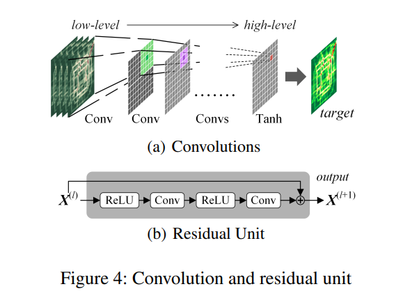
visual rep. of the residual networks - a series of convolutions are used to capture nearbye spatial dependencies.
- stacking convolutions helps to capture distant spatial dependencies since convolutions on low-level features are limited by the size of the kernel.
- convolving over extracted features enables the network to examine higher level features which represent more distant, global relationships in the spatial grid.
- because the network must be deep to represent global patterns, residual connections are used to aid in the training of the model
closeness, period, and trend networks:
- several 2-channel traffic flow matrices of intervals in the respective time are concatenated together along the time axis.
- a convolution operation is conducted over the tensor, and an activation is given to produce the output
- L residual units are then stakced on top of this convolution (see fig 4)
- a final convolution is performed on the output of the L\text{-th} residual unit to obtain the respective time component output
External Component (Fourth)
- three external factors are considered
- holiday event
- weather (thunderstorms, etc.)
- metadata (day of week, weekend, weekday)
- two fc layers are stacked on top the feature vector, E_{t} (contains the external features) for the predicted time interval t
- the first layer embeds each sub-factor and is followed by an activation
- the second layer transforms the low-dimensional representation into a high-dimensional feature tensor X_{Ext} which can be fused with the outputs of the spatial-temporal components, X_{t}
Fusion
- The three temporal X_{t} output tensors are multiplied element-wise by a learned weight tensor, and added together to generate X_{res}
- X_{res} and X_{Ext} are directly fused and run through the Tanh activation function
Loss
The mean squared error is minimized as the goal of optimization for the ST-ResNet model
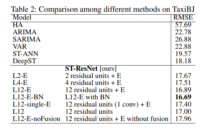
16.1.3 Evaluation
- Datasets:
- TaxiBJ
- BikeNYC
- Compare against the following methods:
- HA: historical average flows
- ARIMA:
- SARIMA: seasonal arima
- VAR
- ST-ANN
- DeepST
16.1.4 Comments
- this is a very good baseline, because it uses primarily convolutional structures which we might be able to implement using a SOTA secure framework, specifically CrypTflow2, which will be another good baseline for comparison
- should be very easy to implement in crypten
16.1.5 Questions
- no questions
16.2 T-Wave
Notes for T-Wave introduced in B. Hui (2021)
16.2.1 Contributions
16.2.2 Methods
16.2.3 Experiments
16.2.4 Questions
- How are trajectory sequences / data actually constructed as inputs to the model?
- How can I obtain access to the code for these models?
- How are the traffic segments structured? They utilize the same methods of dilate spatial temporal convolutions as Graph-WaveNet, but use the trajectory data in order to structure the actual graph data. I don’t really understand their representations too well.
16.3 MA2GCN
Notes on “MA2GCN: Multi Adjacency Relationship Attention Graph Convolutional Networks for Traffic Prediction Using Trajectory Data” Z. Sun (2024)
16.3.1 Contributions
- authors provide methods for converting trajectory-based datasets for traffic flows prediction into graph networks.
- they also provide code implementations
- their graph constructions consider entry and exit matrices for the different grids they construct.
- Their graph analysis framework is extremely similar to graph wavenet, but their adaptive graph generator is unique:
- multi-adjacency relationship attention?
16.3.2 Methods
- utilizes a multi-adjacency relationship attention module to try and accurately learn the spatial information of the input
- focuses on the more important adjacency matrices which are input?
- how many adjacency matrices are input to the model? shouldn’t there be a single matrix representing the entire graph / range of the data or do they divide the data / area of coverage into separate grids and then input them together? The process used here is not very clear.
16.3.3 Experiments / Evaluation
- They use the Shanghai taxi GPS trajectory dataset, and convert it into a graph using their novel trajectory-to-graph conversion methods
- they test their graph convolution routines against state-of-the-art methods for these converted graph data.
- they use the same metrics that all of the GCN analysis papers use. I don’t really like their writeups though. I’m souring on this work a bit. It would be better if we could get access to T-Wave, then we could perform some better analysis on a better model potentially.
16.3.4 Questions
- How is the actual conversion performed? I.e., how does the trajectory data look to start, and how is it converted to a graph format.
- What is the \tilde{X} matrix they metnion in the adaptive graph generator section?
- what is the notation?
- P, D, N, C - what do these symbols denote?
15.4.4 Comments